Handwriting Recognition for Automated Equation Generation

Presentation: https://youtu.be/xZKb-CjaZT8

Introduction + Background

In academia, the document preparation language LaTeX [6] is commonly used to write technical documents and publications. LaTeX code can be tedious to write. Authors can save tremendous amounts of time by being able to convert their handwritten math work directly into LaTeX. Currently, there are many machine learning algorithms being used for text recognition (optical character recognition – OCR [1, 2]), including K-Nearest Neighbors (KNN), neural networks, decision trees, and Support Vector Machines [3]. These algorithms combined with image processing techniques allow for high accuracies of text recognition to be achieved.

While character recognition is well established, there are few handwritten equations to LaTeX algorithms [4, 5]. We propose an OCR framework based on several machine learning techniques, both supervised and unsupervised. First, individual characters are extracted from an input image using the unsupervised clustering algorithm DB SCAN. For unlabeled characters, we explore the use of K-Means and a Gaussian Mixture model to cluster unlabeled characters for convenient manual labeling. Finally, we implement several supervised models to predict characters from images: Decision Trees, Naïve Bayes, and a linear Support Vector Machine (SVM), and two convolutional neural networks trained using Stochastic Gradient Descent.

Problem Definition

This project aims to convert RGB images of handwritten equations into corresponding LaTeX code. Open-source Kaggle datasets for this data are linked in the Data Collection section below. We have divided this problem into several sub-problems. First, we aim to identify individual characters in an image. Second, we aim to assemble the identified characters into an equation. Finally, we aim to systematically convert this representation into the corresponding LaTeX code.

Data Collection

Data for this project consists of two Kaggle datasets. One dataset contains handwritten math symbols with their labels, and the other contains full equations with their corresponding LaTeX representations.

Symbols Dataset: https://www.kaggle.com/xainano/handwrittenmathsymbols

Equation Dataset: https://www.kaggle.com/aidapearson/ocr-data

Methods: Unsupervised Learning

DB SCAN

The first step in the conversion from handwritten text to a formatted equation is to identify the written portions of the image and separate each character into its own feature / image. The amount of information stored in a colorized image is on the order of n×m×3×255, where n and m correspond to the dimensions of the image, 3 related to red, blue, and green layers of the image, which range in value from 0 to 255 (or 8 bits). Grayscale images decrease the complexity by reducing the number of layers to a single layer, however the information stored in this case is still more than necessary. In fact, the complexity of the image can ultimately be reduced into two features: the position of a pixel along the x-axis, and the position of a pixel along the y-axis. This can be attained by converting the image to a binary complement and determining the corresponding position of each pixel.

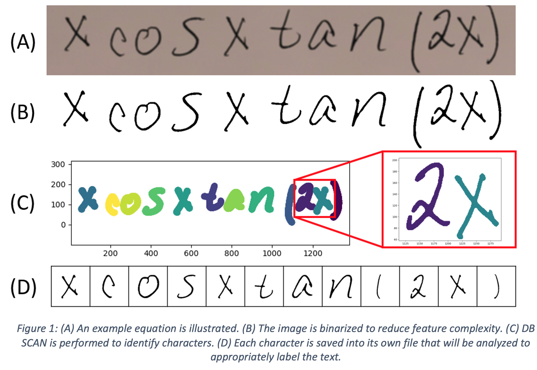
Figure 1 illustrates an example equation, which will be used to demonstrate the machine learning algorithms used in this work. To start, the image is binarized into black and white pixels using an adaptive thresholding technique, which helps to separate the background (white pixels) from the foreground (black pixels) of the image in the event of uneven lighting or light strokes as shown in Figure 1(B). The location of each pixel is converted from a matrix representation, which is used to create an image, to a two-feature array, corresponding to the x and y positions of each foreground pixel. With two features, the data is visualizable and DB SCAN can be performed to begin clustering similar features. DBSCAN is a preferred method of clustering since it does not require the number of clusters in advance, which makes this process more automatable. For this example, an epsilon of 10 pixels and a min_pts of 10 was selected to ensure that the clusters separate into the correct number of characters. However, these values may need to be tuned with images of higher or lower resolution. Once the features are properly segmented, they are converted back to a matrix representation and saved as individual square images for uniformity and normalization.

Feature Engineering

Supervised methods require labeled training data for effective classification. However, manually labeling characters can be tedious and time-consuming. By clustering variations of the same character into groups, each cluster can be quickly and conveniently. For example, in Figure 1, three characters are “x”, which will all share features and characteristics that help distinguish them from other characters in the equation. Clustering algorithms allow us to group characters with similar features. Due to the large number of pixels in each image, it is beneficial to reduce the complexity of each image by identifying features in the image that are unique to that character.

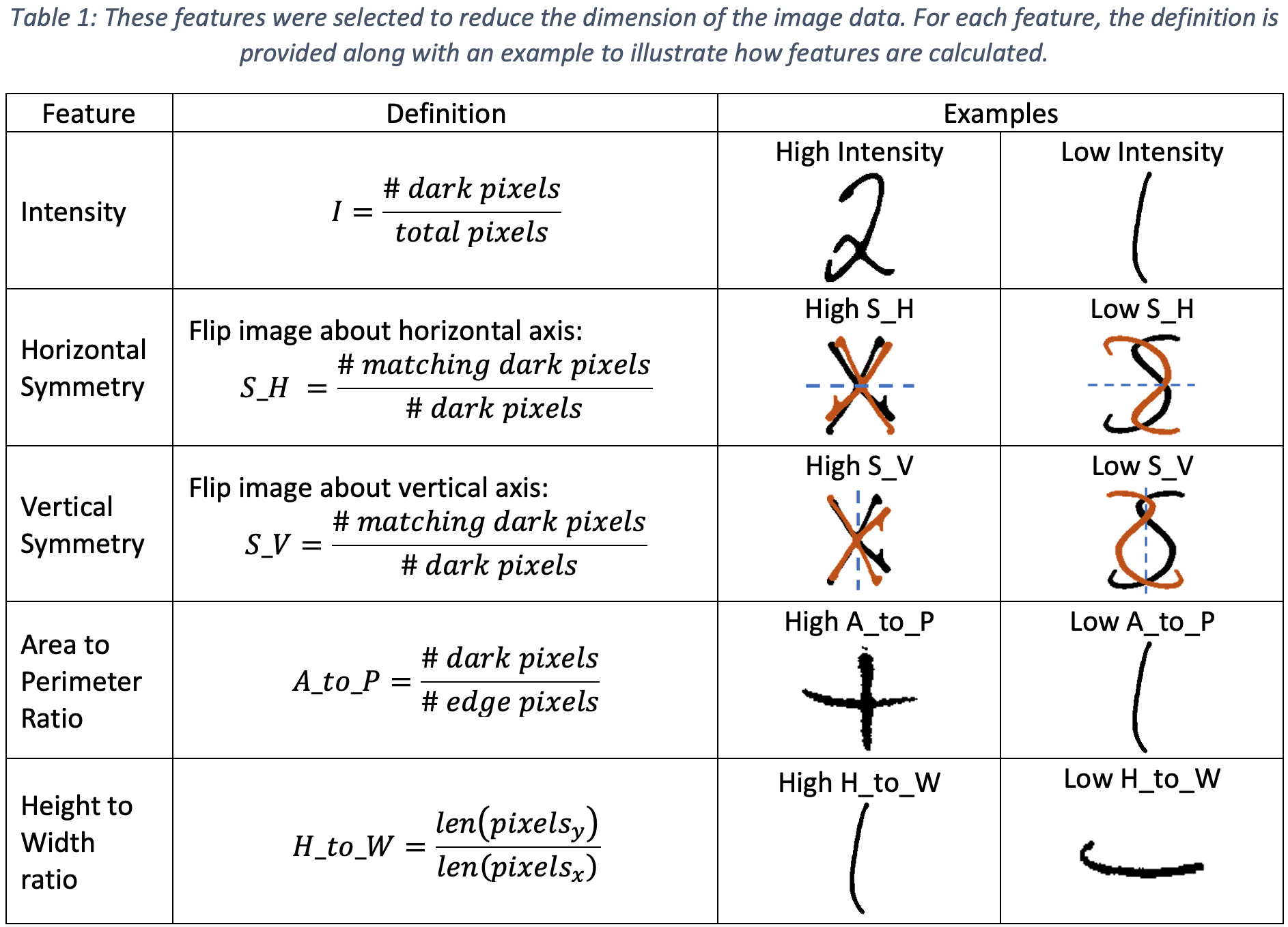
Feature engineering, in which metrics are developed to describe certain properties of the image, offers one approach to identifying features. Table 1 provides the features that were engineered for clustering. These features were extracted from handwritten letters and clustering was performed to effectively separate unique characters. However, these features generally resulted in poor clustering performance, as the chosen set of features was not informative enough to provide any clear separation between different characters. This is likely because of high variations in the style of writing different characters. Furthermore, this form of feature engineering requires manual design of the features. Features designed for a particular dataset may not generalize well and may thus require a manual redesign for each new dataset.

Principal Component Analysis (PCA)

Principal Component Analysis (PCA) offers a more intelligent way to determine which features are most important for identifying characters. Treating each image pixel as a feature, PCA can be used to determine the linear combinations of pixel values that will be most useful for identifying characters. PCA achieves this by maximizing the variance of the transformed data along each principal component. Thus, the principal components represent the linear combinations of pixel values that have the most variation, which distinguishes them from other characters. After performing PCA, the scores of the data along the two largest principal components can be used as features for clustering. In this way, informative features are learned from the dataset automatically.

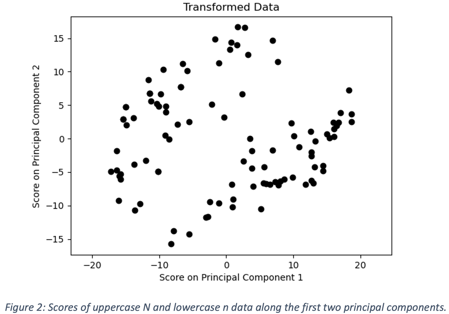
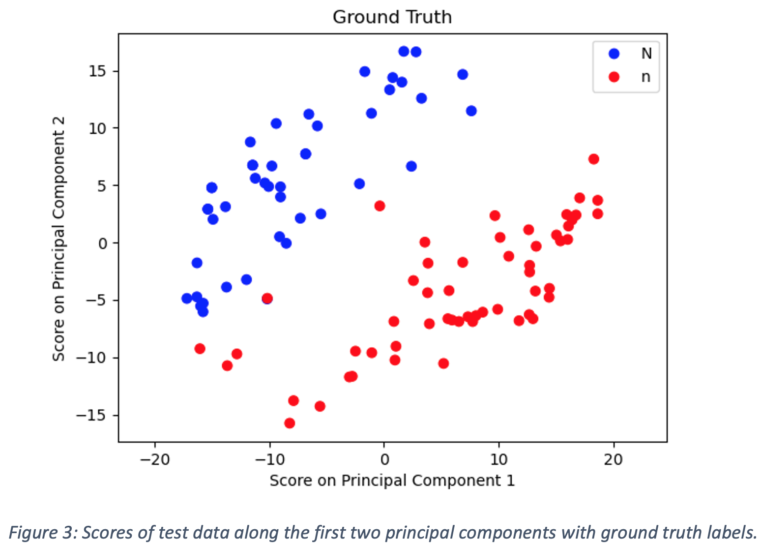
One of the weaknesses discovered in the symbol dataset was that uppercase and lowercase versions of the same letter were given the same label. In the context of converting handwritten equations to LaTeX, the distinction letter case is important. As previously noted, manually labeling characters can be significantly simplified by grouping the characters into separate clusters. To test the performance of our feature identification via PCA and subsequently presented clustering algorithms, we use a manually labeled reduced dataset of 100 images containing 50 images each of the uppercase letter “N” and the lowercase letter “n”. The scores of the data on the two largest principal components are shown below in Figure 2. The first two principal components explain 21.8% and 10.6% of the variance respectively. The ground truth labels are provided in Figure 3 and demonstrate that PCA successfully separates the characters.

K-Means Clustering

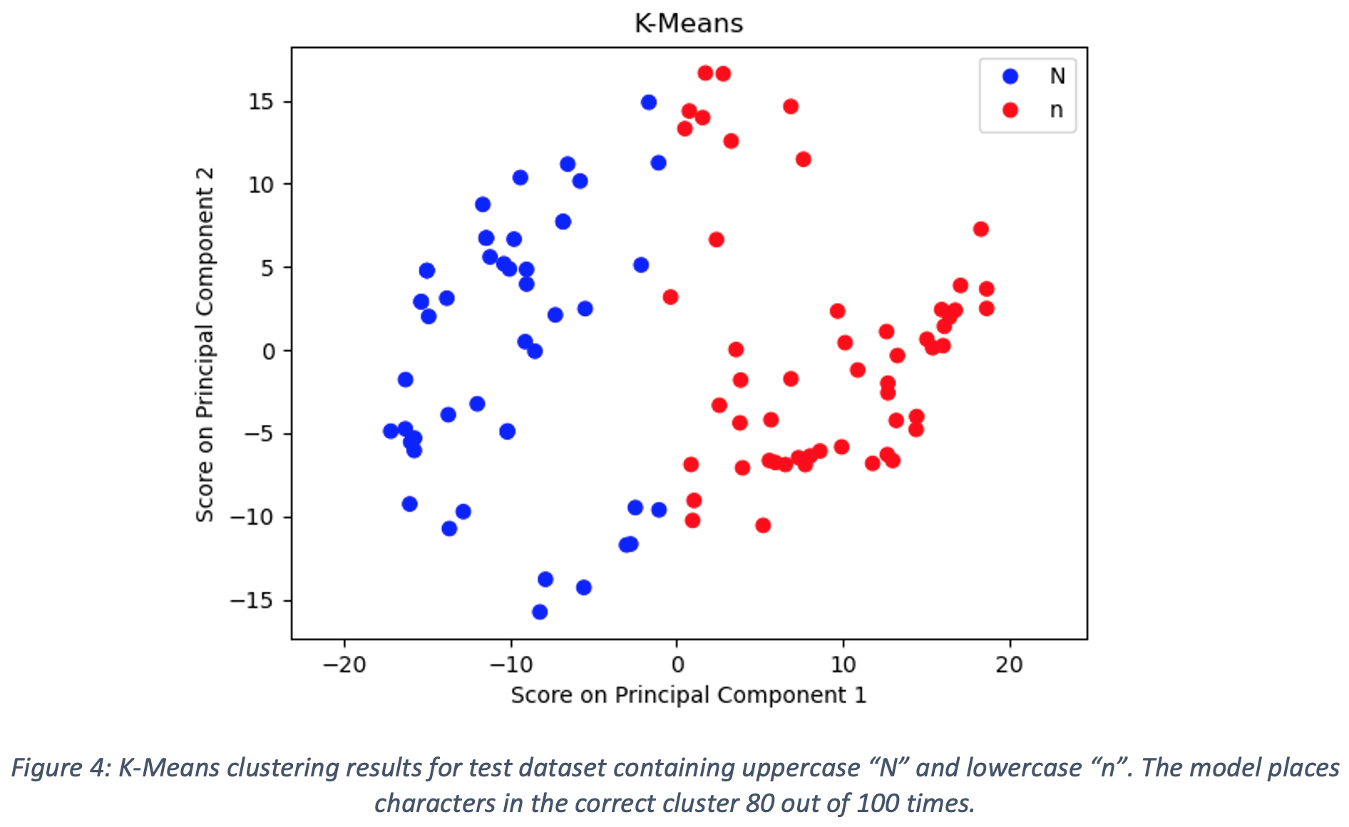
The first clustering algorithm employed was K-Means with the number of clusters set to 2 and the means initialized randomly. The results of the K-means clustering on the test dataset are shown in Figure 4. Blue points are classified as uppercase N while red points are classified as lowercase n. K-Means places characters in the correct cluster 80 out of 100 times for the test dataset. There are several instances of both uppercase N characters being placed in the lowercase n cluster and lowercase n characters being placed in the uppercase N cluster. The majority of the error associated with the K-Means clustering for the test dataset stems from the inability of the algorithm to recognize the underlying distributions of the transformed data for each character. Since K-Means has no knowledge of these underlying distributions, it cannot leverage the fact that the scores on the first two principal components are clearly correlated for both characters. Without this information, the clustering assumes no correlation and splits the data left and right. While using K-Means to split the characters into groups does outperform random division into groups, utilizing knowledge of the underlying distributions can further improve clustering performance.

Gaussian Mixture Model (GMM)

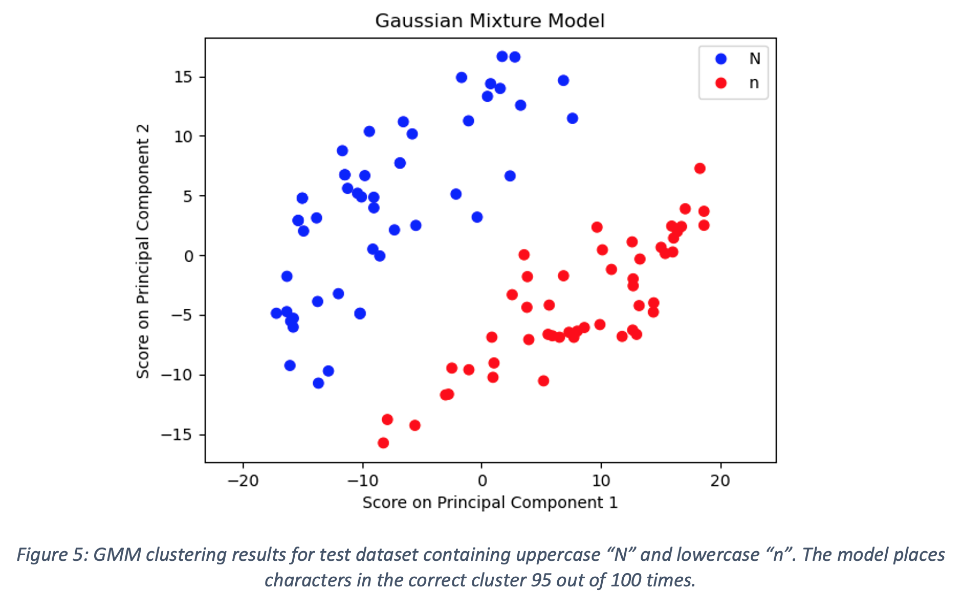
After pinpointing the weaknesses associated with the use of K-Means clustering for the test dataset, the next algorithm employed was a Gaussian Mixture Model (GMM) with the number of components set to 2 and the means and covariances initialized using the results of the K-Means clustering. As GMM is a soft clustering algorithm, datapoints were assigned to the cluster with the highest probability given the datapoint. The results of the GMM clustering on the test dataset are shown in Figure 5. Blue points are classified as uppercase N while red points are classified as lowercase n. GMM places characters in the correct cluster 95 out of 100 times for the test dataset. All errors were cases in which a lowercase n was placed in the uppercase N cluster. The small number of datapoints and consistency of the error suggest that a certain small percentage of lowercase n characters share some properties of uppercase N characters. It should also be noted that each of the incorrectly clustered points lie close to the decision boundary. Although not perfect, GMM is able to outperform K-Means by leveraging knowledge of the covariance between the scores on the first two principal components.

Methods: Supervised Learning

Image Preparation for Traditional Machine Learning Models

The goal of the supervised learning here was to build a model which could identify the symbol contained within an image. To train models, the symbols dataset was used, which contained 350,000+ images, split into training (70%) and testing (30%) datasets. Each image was preprocessed by resizing and thresholding to reduce the number of pixels in each image to speed up training.

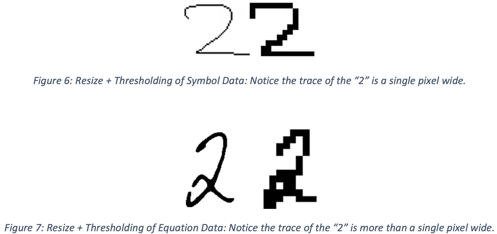
Each square (45x45 pixels) grayscale image (containing a single symbol) was resized to 24x24 pixels, followed by thresholding operation, then resized to 12x12 and thresholded to binarize the image while retaining the shape of the original symbol. This was done to improve the similarity of the symbols dataset and the equations dataset. By thresholding, variations in grayscale values are removed, reducing noise in the data. Examples of processed symbol images are shown in Figure 6 and Figure 7. A Decision Tree, linear SVM (Stochastic Gradient Descent classifier), and Naive Bayes model were trained with each pixel representing a feature of the data (for a total of 144 features per image) using sklearn models.

Convolutional Neural Network Architecture and Image Augmentation

ResNet18

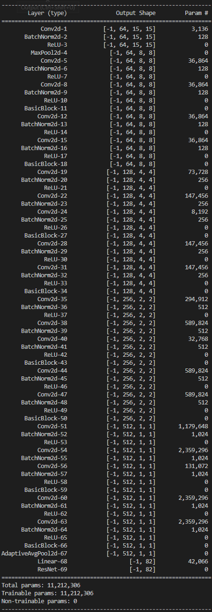
A convolutional neural network (CNN) was trained to improve upon the traditional supervised methods. This CNN was based on the ResNet18 (PyTorch, 2022) architecture, with a modified Conv2D input (which accepted a grayscale rather than RGB image) and modified output (82 output layers, one for each symbol class). The network contained a total of 69 layers and 11,212,306 parameters, as shown in Appendix A.

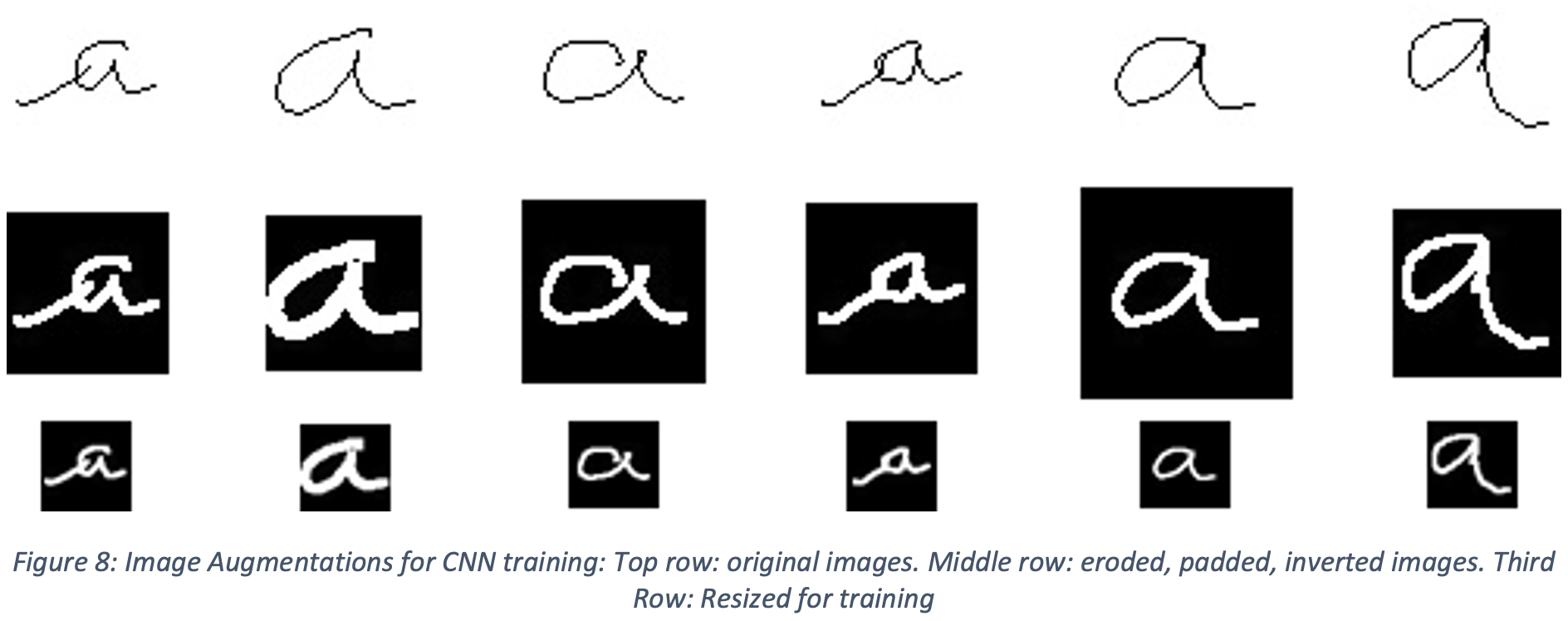
Prior to training the network, in order to help with generalization, the dataset was augmented with random permutations. First, the trace of the symbol within each 45x45 pixel image was randomly eroded (enlarging the black areas and increasing the line width) between 1 and 4 times. Then the image was padded with between 2 and 12 pixels (resulting in images ranging in size from 49x49 pixels to 59x59 pixels). These images were then binarized, black/white inverted, and finally rescaled to 30x30 images, as shown in Figure 8.

During training, the Adam optimizer was selected. The first 5 epochs were initialized with a learning rate of 0.003. The final 5 epochs were initialized with a learning rate of 0.0003, which was found to help the network move from 96.5% accuracy to 97.5%.

Custom Multilayer CNN

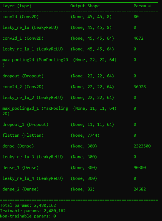
A second, simpler CNN was created to examine the effects of reducing the number of parameters used during training on the final accuracy of the model. This CNN had just 16 layers and 2,480,162 parameters, as shown in Appendix A. LeakyReLU was chosen as the activation function for all layers.

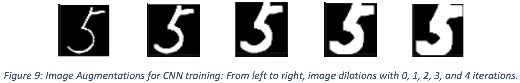
Prior to training, the dataset used for this model also underwent some image preprocessing. In this model, the images used for training were first inverted and then dilated to thicken the trace of the symbols. Each of the images were dilated a random iteration number of times between 0 and 4, as shown in Figure 9. This produced a greater variation in the data used in training that can help the model better generalize. The images were then normalized by dividing the entire image array by 255.

During training, the stochastic gradient descent optimizer was used for a total of 5 epochs with a learning rate of 0.01 and momentum of 0.9.

Results and Discussion

Unsupervised Learning

For clustering pixels which belong to a single character, DBSCAN performed well under ideal circumstances. However, we identified a key failure mode for this method. Characters with multiple separate markings, such as “i” and “=” cannot be consistently identified using DBSCAN alone. Therefore, an additional script was implemented to concatenate images with similar vertical position. For characters consisting of connected markings, DBSCAN is effective for identification and noise removal. While DBSCAN was effective, there are simpler methods which can achieve similar results. Because the pixels are evenly spaced and the image is binarized, DBSCAN is effectively performing simpler blob detection, such as those found in [7]. However, if clustering is performed on a higher resolution image with more noise, performing DBSCAN with a larger radius may effectively cluster across small, unintentional gaps in handwritten text.

For clustering characters, feature engineering presented challenges. These challenges were addressed through the use of PCA, which allowed for a more effective feature engineering process that could also be automated. K-Means clustering of characters provided an improvement over random division into groups but suffered from an inability to identify the underlying distributions associated with the transformed data for each character. GMM leveraged knowledge of the correlation between features to achieve an improved clustering compared to K-Means.

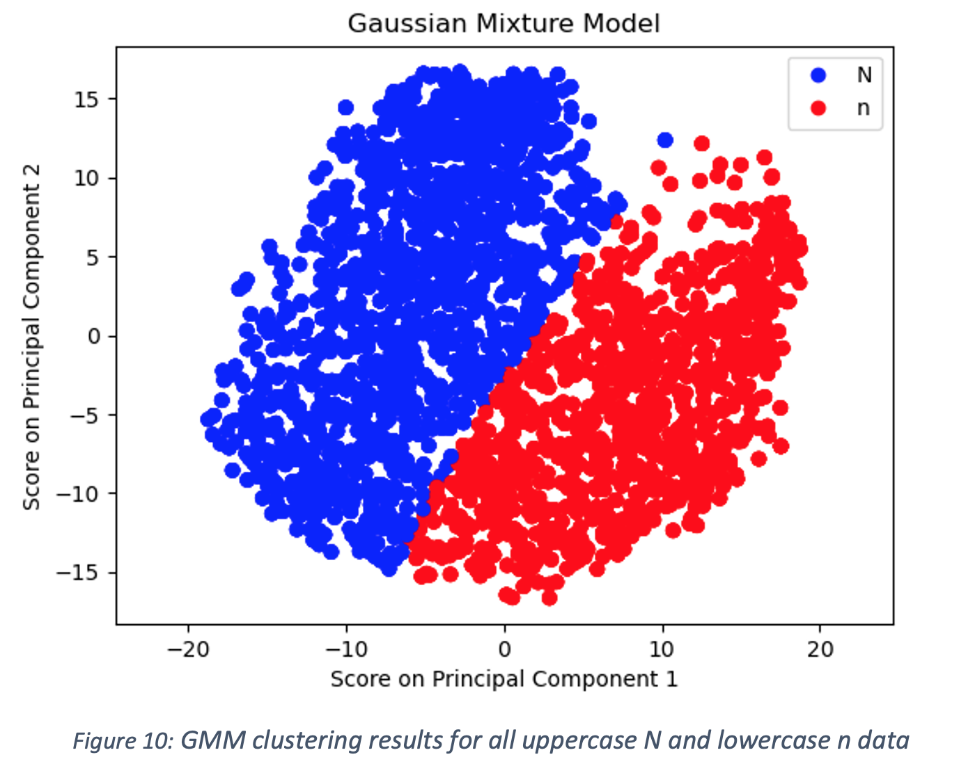
While the combined use of PCA and GMM achieved good clustering performance on the smaller test dataset, it did not generalize well to the larger dataset. This can likely be attributed to the fact that the larger dataset contains significantly more images and variations of letters. Additionally, test images were selected manually and were thus more likely to be easily identifiable, while the larger dataset likely has significantly more edge cases and thus more variance. This is reflected in the clustering results provided below using all the data for uppercase N and lowercase n rather than just a subset. The PCA was unable to clearly separate the two groups, leading to poor GMM clustering performance.

Supervised Learning

Decision Tree

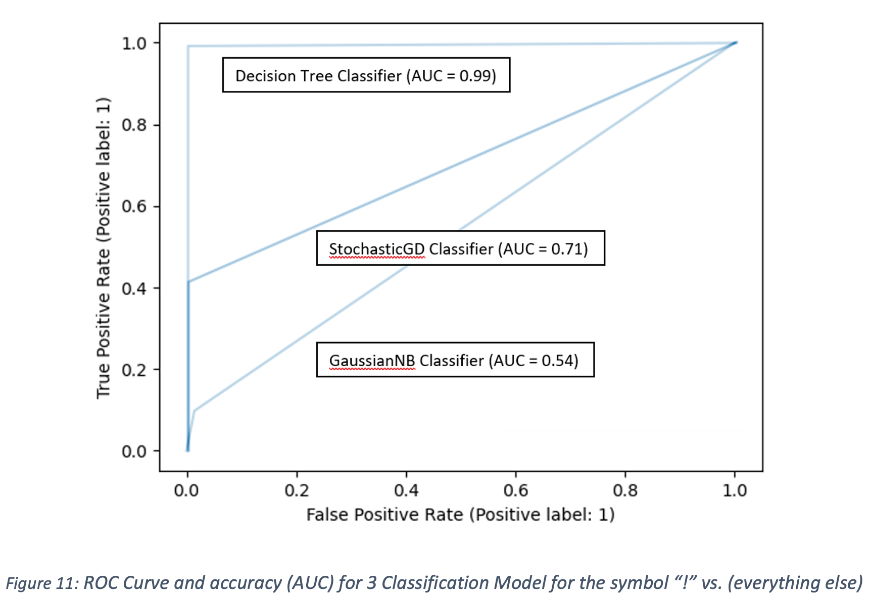
The traditional supervised learning method that yielded the best results was the Decision Tree Classifier. As seen from Figure 11, the area under the curve for the ROC plot of the Decision Tree Classifier was 0.99 for the classification of the symbol “!” (results are representative of all results for each label). This score was achieved using the test portion of the symbols dataset. However, when the Decision Tree model was used on the images from the output of the image segmentation from the equations dataset, the model performed poorly, with less than 25% accuracy on the equations dataset. This indicates that the pre-processing of the individual symbol dataset did not produce a dataset which led to a generalized model. Thus, additional pre-processing work is required for satisfactory results, which are explored further in building a convolutional neural network.

ResNet18

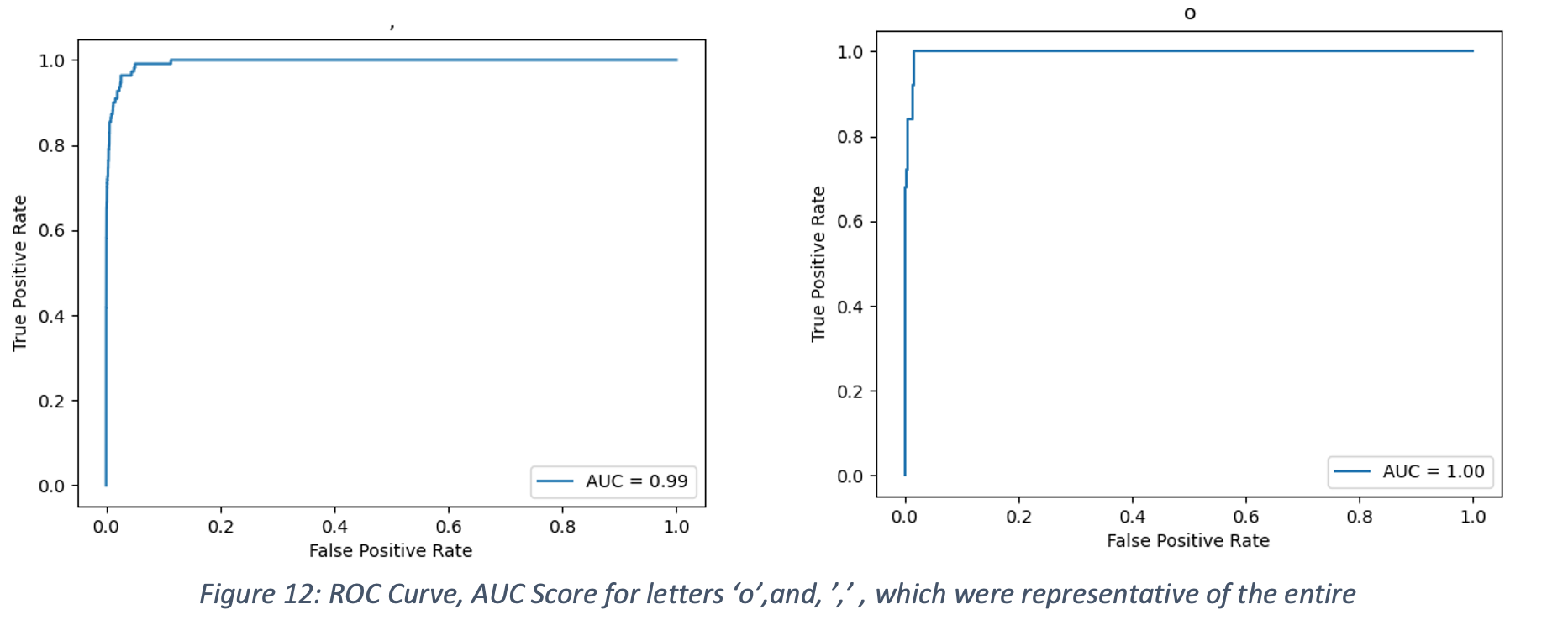
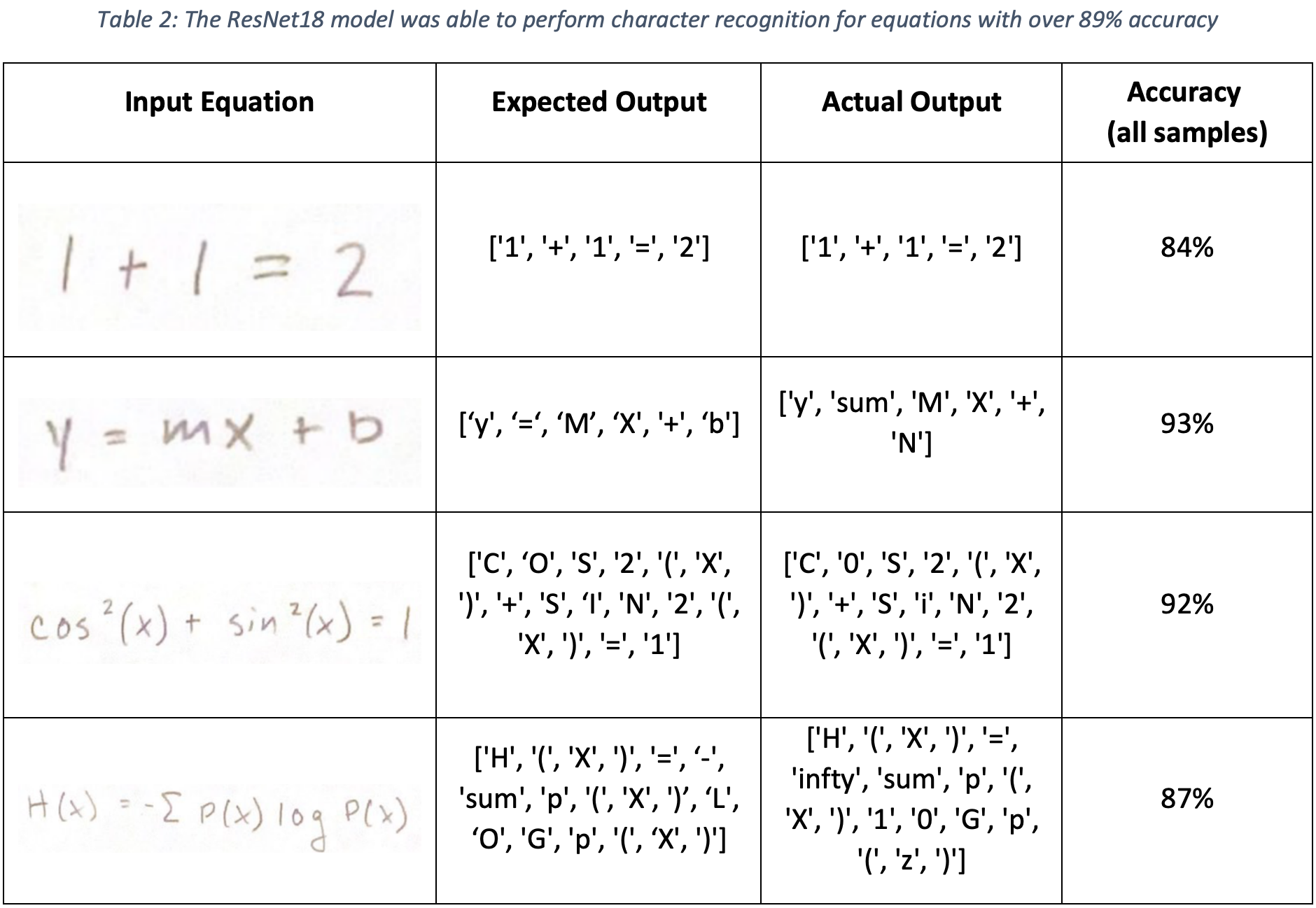
After 10 epochs of training, the ResNet18 Convolutional Neural Network (CNN) demonstrated 97.5% accuracy during validation. Furthermore, the average AUC score was 0.99, as shown in Figure 12. Testing on the handwritten equation dataset (after separating out each symbol using the DB SCAN method), produced overall prediction accuracy was 89.13%, with samples shown in Table 2.

Custom Multilayer CNN

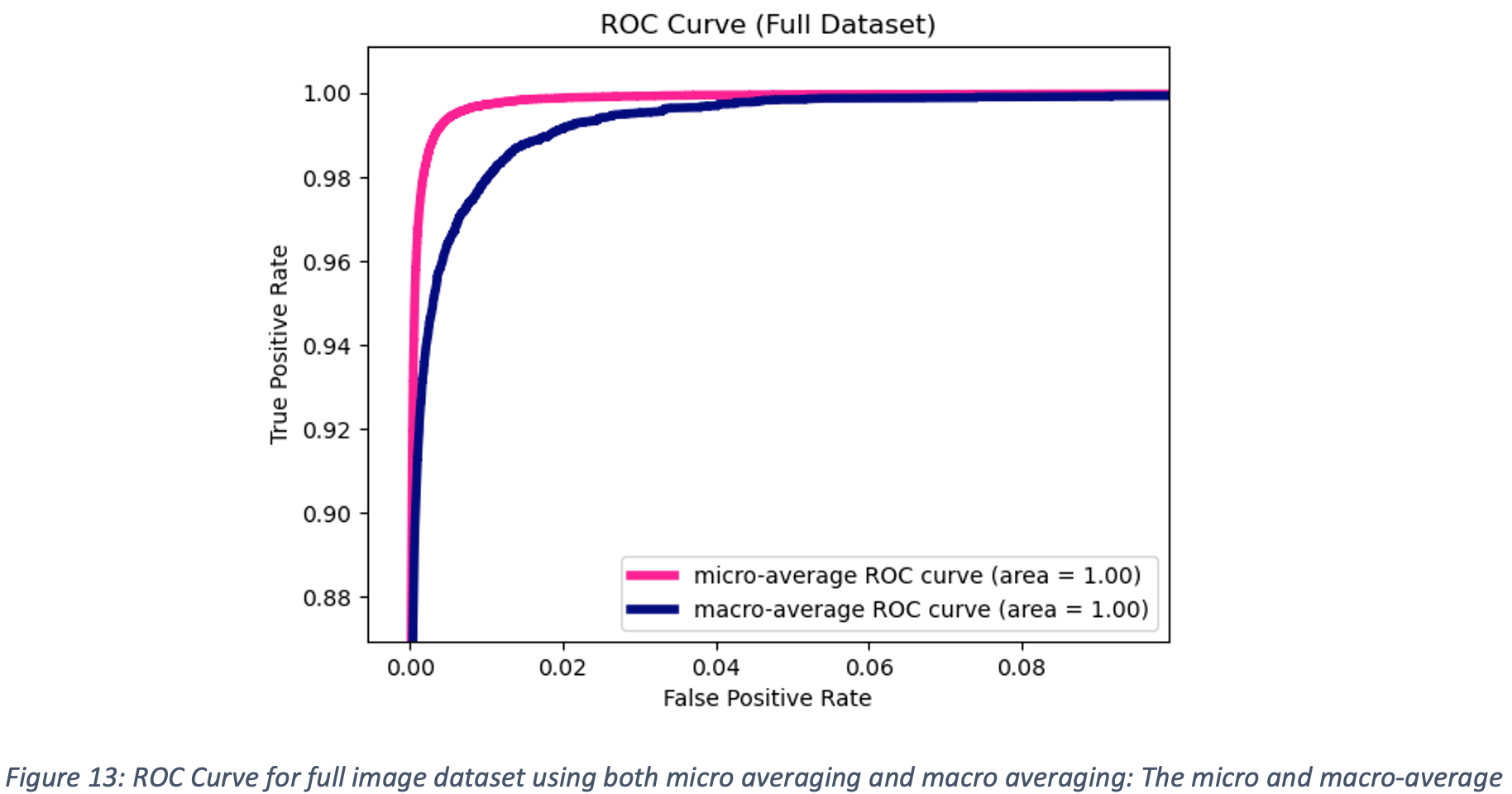
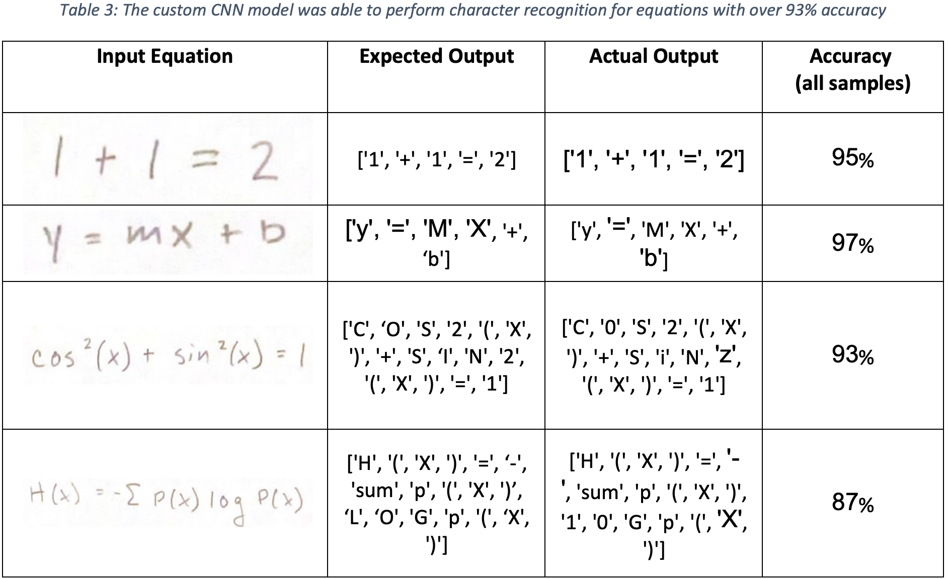
After just 3 epochs of training, the custom built Convolutional Neural Network (CNN) demonstrated 94.9% accuracy during validation. A micro-average and macro-average ROC curve were plotted for the model evaluation, and the AUC score for both was 0.99, as shown in Figure 13. Testing on the handwritten equation dataset (after separating out each symbol using the DB SCAN method), produced overall prediction accuracy was 93%, with samples shown in Table3. Surprisingly, the Custom CNN performed better than the ResNet18 CNN. This may be attributed to the differences in the dataset used to train both models. For the Custom CNN, the image data was augmented to randomly thicken the trace of the symbols. This introduced a greater variation into the dataset which helped the model generalize better. Even though the Custom CNN model was much simpler than the ResNet18 model, the overall better performance may partially be attributed to the different quality of images used to train the Custom CNN model. This highlights the importance of data used to train a model, as the model predicted results will only be as good as the data it was trained on.

LaTeX Equation Reconstruction

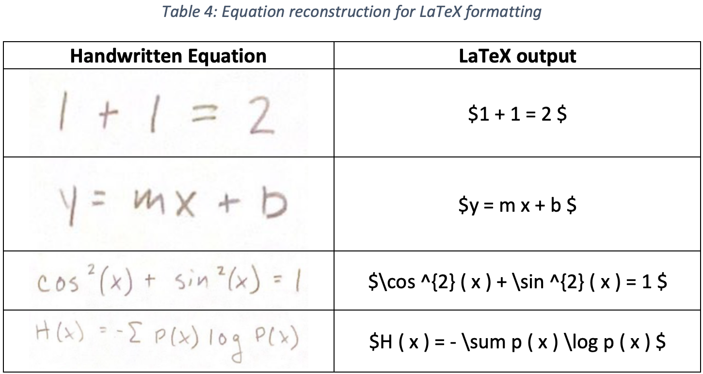
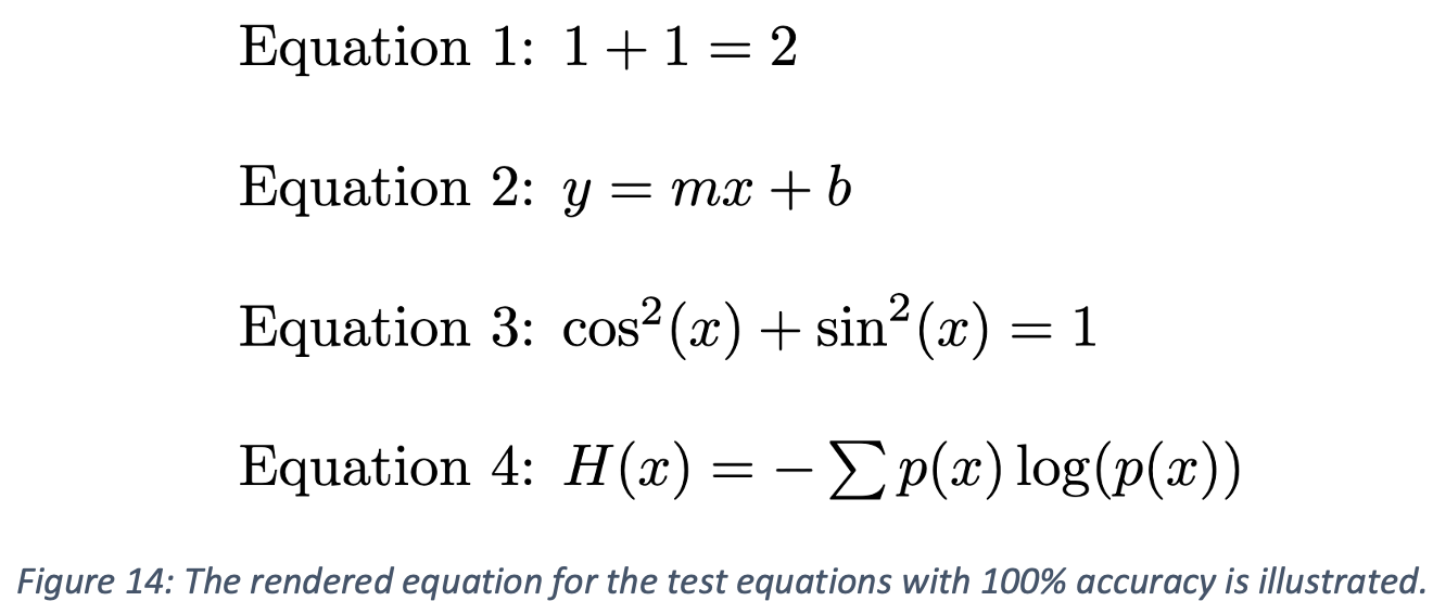
After classifying each character in the equation, the corresponding LaTeX code can be generated. First, the characters in the equation are sorted from left to right based on the location of the bottom corner of the blob identified using DB SCAN. Then, exponents are identified by checking the height change between consecutive characters. A threshold of 50 pixels height change in the raw input image was selected to identify exponents. Characters such as “+” and “=” are ignored during the exponent check. Lastly, the software checks for control sequences in the equation and replaces them with their corresponding commands. For example, three consecutive characters “L-O-G” would be replaced with the control sequence “\log” in the output. An example implementation is shown in the code included in the Appendix A. This system successfully reconstructed the LaTeX equations for several test cases, as shown in Table 4. Rendered LaTeX script using this output is shown in Figure 14.

Conclusion

Through the application of machine learning and image processing techniques, an accurate mathematical symbol recognition system was developed. The pipeline for this system is first image segmentation, symbol identification, and finally conversion to LaTeX. Image segmentation was done using the unsupervised learning algorithm DBSCAN on a single line mathematical expression to separate and pull out each individual symbol within the overall expression. Symbol identification was achieved with Convolutional Neural Networks, where an 82-label neural network model was fit to the training image data. Finally, a python script was used to convert the outputs of the CNN model into Latex formatting.

In the future, this model could be improved by implementing a time-dependent structure, which identifies the character as well as the sequence of the character for better equation recognition. Additionally, the model could be trained on entire equations rather than single characters. These improvements will give the network a better understanding of the intent of intent of the character and may help improve accuracy between distinguishing characters such as “0” (zero), “o” (lowercase o), and “O” (uppercase O). Finally, with further development to the pre and post processing of images, this system may be able to format more complex or multi-line equations.

References

[1] R. Smith. An Overview of the Tesseract OCR Engine, Proceedings of the Ninth International Conference on Document Analysis and Recognition (ICDAR 2007) Vol 2 (2007), pp. 629-633.

[2] Naz, S., Umar, A.I., Shirazi, S.H. et al. Segmentation techniques for recognition of Arabic-like scripts: A comprehensive survey. Educ Inf Technol 21, 1225–1241 (2016). https://doi.org/10.1007/s10639-015-9377-5

[3] J. Memon, M. Sami, R. A. Khan and M. Uddin, “Handwritten Optical Character Recognition (OCR): A Comprehensive Systematic Literature Review (SLR),” in IEEE Access, vol. 8, pp. 142642-142668, 2020, doi: 10.1109/ACCESS.2020.3012542.

[4] Kröger, O. (2018, August 18). Handwritten equations to latex. OpenSourc.ES. Retrieved February 21, 2022, from https://opensourc.es/blog/he2latex/

[5] Wang, H., & Shan, G. (2020, February 26). Recognizing handwritten mathematical expressions as latex sequences using a multiscale robust neural network. arXiv.org. Retrieved February 21, 2022, from https://arxiv.org/abs/2003.00817

[6] “An introduction to LaTeX”. LaTeX project. Retrieved 18 April 2016.

[7] Shneier, Michael. “Using pyramids to define local thresholds for blob detection.” IEEE transactions on pattern analysis and machine intelligence 3 (1983): 345-349.

Appendix A

ResNet18 Architecture

Custom CNN Architecture

LaTeX Writer Class

import numpy as np

class Character:
    def __init__(self, character_id, pos):
        self.character_id = character_id
        self.pos = pos

class LaTeXFeatures:
    def __init__(self):
        self._frac = '\ frac'.replace(" ","")
    
    def curly(self, x):
        return "{" + str(x.character_id) + "}"

    def frac(self, x, y):
        return '{}{}{}'.format(self._frac, self.curly(x), self.curly(y))

    def exp(self, x):
        return "^" + self.curly(x)

class LaTeXWriter:
    def __init__(self):
        self.features = LaTeXFeatures()
        self.control_sequences = ["sin", "cos", "sum", "log"]
        self.exp_excluded_chars = ["+", "-", "=", "."] # exclude small characters - may be buggy for "-"
        self.exp_height = 50

    def sort_characters_lr(self, characters):
        character_positions = np.array([character.pos for character in characters])
        sorted_ids = np.argsort(character_positions[:, 0])
        new_characters = []
        for i in sorted_ids:
            new_characters.append(characters[i])
            
        return new_characters

    def get_character_sequence(self, characters):
        character_sequence = ""
        for character in characters:
            character_sequence += character.character_id
        
        return character_sequence

    def get_character_start_indices_in_sequence(self, characters):
        # useful when characters have character_ids longer than 1
        start_indices = []
        i = -1
        for character in characters:
            j = len(character.character_id)
            i += j
            start_indices.append(i)
        return start_indices

    def check_for_sequence(self, characters, sequence):
        character_sequence = self.get_character_sequence(characters)
        sequence_start = -1
        single_char = False

        if sequence in character_sequence:
            pos = character_sequence.find(sequence)
            # print("Sequence " + sequence + " found at position " + str(pos))
            sequence_start = pos
        
            # check if sequence is in any single character
            for i in range(len(characters)):
                character = characters[i]
                if character.character_id == sequence:
                    sequence_start = i - 1
                    single_char = True
        
        return sequence_start, single_char
    
    def write_equation(self, characters):
        characters = self.sort_characters_lr(characters)
        character_start_indices = self.get_character_start_indices_in_sequence(characters)
        eqn_string = "$"

        # check for control sequences
        for control in self.control_sequences:
            sequence_start, single_char = self.check_for_sequence(characters, control)

            # check if sequence found; -1 indicates not found
            # extra logic for handling if a control sequence is inside a single char
            if sequence_start >= 0:
                char_indices = np.where(np.array(character_start_indices) == sequence_start)[0]
                for i in range(len(char_indices)):
                    char_index = np.asscalar(char_indices[i])
                    if single_char:
                        char_index += 1
                    new_id = "\\" + control
                    new_char = Character(new_id, characters[char_index].pos)
                    n_characters = len(control)
                    end_start = char_index + n_characters - len(control) + 1 if single_char else char_index + n_characters
                    characters = characters[:char_index] + [new_char] + characters[end_start:]

            # recompute starts
            character_start_indices = self.get_character_start_indices_in_sequence(characters)

        for i in range(len(characters)):
            character = characters[i]

            (x, y) = character.pos

            if i > 0:
                prev_character = characters[i - 1]
                (x_prev, y_prev) = prev_character.pos

                # check if exponent
                if -(y - y_prev) > self.exp_height and characters[i].character_id not in self.exp_excluded_chars:
                    eqn_string += self.features.exp(character)
                else:
                    eqn_string += character.character_id

            else:
                eqn_string += character.character_id
            
            eqn_string += " "

        eqn_string += "$"
        return eqn_string

Example LaTeX Conversion Code

writer = LaTeXWriter()
height = 10
exp_height = -(height + 50 + 1)

# Equation 3: cos^2(x) + sin^2(x) = 1
# Character arguments: Character(character_id, character_position)
c = Character("c", [0, height])
o = Character("o", [1, height])
s_1 = Character("s", [2, height])
two_1 = Character("2", [3, exp_height])
open_1 = Character("(", [4, height])
x_1 = Character("x", [5, height])
close_1 = Character(")", [6, height])
plus = Character("+", [7, height])
s_2 = Character("s", [8, height])
i = Character("i", [9, height])
n = Character("n", [10, height])
two_2 = Character("2", [11, exp_height])
open_2 = Character("(", [12, height])
x_2 = Character("x", [13, height])
close_2 = Character(")", [14, height])
equals = Character("=", [15, height])
one = Character("1", [16, height])

eq3 = [c, o, s_1, two_1, open_1, x_1, close_1, plus, s_2, i, n, two_2, open_2, x_2, close_2, equals, one]
string_eq3 = writer.write_equation(eq3)
print("Equation 3:")
print(string_eq3)
print(" ")
print("\\bigskip")

Proposal Items

Resources from the project proposal can be found below.

Proposal Video Link

https://youtu.be/yFlKFNbGy1g

Timeline and Responsibilities

GANTT Chart: PDF

Excel